H1st Oracle: Combine Encoded Domain Knowledge with Machine Learning
In this tutorial, we will demonstrate the end-to-end process of building Oracle, from raw data to Oracle model, using Microsoft Azure Predictive Maintenance dataset. Through this tutorial, you will learn 1. how to build rule-based model through data analysis 2. how to build Oracle from this rule-based model and your unlabeled data. You can find the notebook version of this tutorial here.
This tutorial has the following contents.
1. H1st Oracle - What is H1st Oracle? - Architecture of Oracle
2. Setup an Experiment - Define the problem we solve in this tutorial - Experiment Process
3. Microsoft Azure Predictive Maintenance dataset - Show basic Exploratory Data Analysis (EDA) - Find some rules (patterns) that can be used to predict faulty components of a machine
4. Build a rule-based Model - Build a rule-based model that can predict the faulty component of a machine - Evaluate the performance of a rule-based model
5. Build an Oracle using H1st.TimeSeriesOracle class - From a rule-based Fault Predictor, build an Oracle - Evaluate the performance of Oracle and compare it with that of rule-based model
1. H1st Oracle
1.1 What is H1st Oracle ?
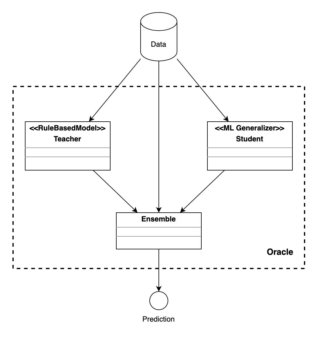
Oracle is a special form of Knowledge-First AI in H1st. It helps you combine your rule-based model with Machine Learning (ML) approach. More specifically, from the rule-based model (Teacher) that you provided, H1st Oracle autogenerates multiple ML Generalizers (Students) and combine those Teacher and Students using Ensemble technique. Through this Oracle approach, you can build ML models without using any labeled data. Furthermore, your AI performance will keep improving as you collect more data from a deployed AI system without updating your existing rules (of course you can update and add more rules, but you don’t need to). Lastly, if you already have some labeled data, you can use them as well to build a more powerful Oracle.
1.2 Architecture of Oracle
Oracle consists of one Teacher (RuleBasedModel), multiple Students (ML Generalizer), and one Ensemble.
Additionally:
* To learn more about H1st framework, please visit h1st.ai
* You can also check out the H1st API documentation
2. Setup an Experiment
2.1 Define the problem we solve in this tutorial
In this tutorial, we want to solve Predictive Maintenance problem. Predictive Maintenance is to help determine the condition of operating equipments and proactively suggest when and what parts of equipment require maintenance work. In this tutorial, we will narrow down the problem and focus on identifying what part of equipment is going to fail and, therefore, need to be replaced. We can go deeper into this problem and differentiate “predicting the potential failure of component of not yet failed machine” and “(postmortem) predicting a root cause component of failed machine”. However, for simplicity, here we will consider them as the same problem.
One important aspect of Oracle that we have emphasized is that we can build Oracle without any labeled data. In this tutorial, we use labeled data (machine failure records) only to create rules (patterns) for detecting component failure. If we had domain knowledge on this Microsoft Azure equipments, we wouldn’t have used any labeled data to create rules.
2.2 Experiment Process
The experiment process will be like the following.
Through data analysis, identify rules and build a rule-based model that can classify faulty component of machine
Split the entire dataset into training set and test set.
Evaluate the rule-based model using test set.
Build Oracle using the rule-based model and training set (without label)
Evaluate the Oracle using test set.
Compare the evaluation results of rule-based model and Oracle
3. Microsoft Azure Predictive Maintenance dataset
In this section, we will do basic Exploratory Data Analysis (EDA) to find out some rules (patterns) that can be used to predict potentially faulty components of a machine. We load the Microsoft Azure sample data and create Pandas DataFrame objects for EDA.
Description of the dataset
We got the the following details of the dataset from https://www.kaggle.com/arnabbiswas1/microsoft-azure-predictive-maintenance
Telemetry Time Series Data (PdM_telemetry.csv): It consists of hourly average of voltage, rotation, pressure, vibration collected from 100 machines for the year 2015.
Error (PdM_errors.csv): These are errors encountered by the machines while in operating condition. Since, these errors don’t shut down the machines, these are not considered as failures. The error date and times are rounded to the closest hour since the telemetry data is collected at an hourly rate.
Maintenance (PdM_maint.csv): If a component of a machine is replaced, that is captured as a record in this table. Components are replaced under two situations: 1. During the regular scheduled visit, the technician replaced it (Proactive Maintenance) 2. A component breaks down and then the technician does an unscheduled maintenance to replace the component (Reactive Maintenance). This is considered as a failure and corresponding data is captured under Failures. Maintenance data has both 2014 and 2015 records. This data is rounded to the closest hour since the telemetry data is collected at an hourly rate.
Failures (PdM_failures.csv): Each record represents replacement of a component due to failure. This data is a subset of Maintenance data. This data is rounded to the closest hour since the telemetry data is collected at an hourly rate.
Metadata of Machines (PdM_Machines.csv): Model type & age of the Machines.
Acknowledgements
This dataset was available as a part of Azure AI Notebooks for Predictive Maintenance. But as of 15th Oct, 2020 the notebook is no longer available. However, the data can still be downloaded using the following URLs: https://azuremlsampleexperiments.blob.core.windows.net/datasets/PdM_telemetry.csv https://azuremlsampleexperiments.blob.core.windows.net/datasets/PdM_errors.csv https://azuremlsampleexperiments.blob.core.windows.net/datasets/PdM_maint.csv https://azuremlsampleexperiments.blob.core.windows.net/datasets/PdM_failures.csv https://azuremlsampleexperiments.blob.core.windows.net/datasets/PdM_machines.csv
3.1 Exploratory Data Analysis (EDA)
import pandas as pd
import plotly.express as px
data_basepath = 'https://azuremlsampleexperiments.blob.core.windows.net/datasets/'
df_telemetry = pd.read_csv(data_basepath + 'PdM_telemetry.csv')
df_telemetry.shape
(876100, 6)
df_telemetry.head()
| datetime | machineID | volt | rotate | pressure | vibration | |
|---|---|---|---|---|---|---|
| 0 | 2015-01-01 06:00:00 | 1 | 176.217853 | 418.504078 | 113.077935 | 45.087686 |
| 1 | 2015-01-01 07:00:00 | 1 | 162.879223 | 402.747490 | 95.460525 | 43.413973 |
| 2 | 2015-01-01 08:00:00 | 1 | 170.989902 | 527.349825 | 75.237905 | 34.178847 |
| 3 | 2015-01-01 09:00:00 | 1 | 162.462833 | 346.149335 | 109.248561 | 41.122144 |
| 4 | 2015-01-01 10:00:00 | 1 | 157.610021 | 435.376873 | 111.886648 | 25.990511 |
df_machines = pd.read_csv(data_basepath + 'PdM_machines.csv')
df_machines.shape
(100, 3)
df_machines.head()
| machineID | model | age | |
|---|---|---|---|
| 0 | 1 | model3 | 18 |
| 1 | 2 | model4 | 7 |
| 2 | 3 | model3 | 8 |
| 3 | 4 | model3 | 7 |
| 4 | 5 | model3 | 2 |
df_failures = pd.read_csv(data_basepath + 'PdM_failures.csv')
df_failures.shape
(761, 3)
df_failures.head()
| datetime | machineID | failure | |
|---|---|---|---|
| 0 | 2015-01-05 06:00:00 | 1 | comp4 |
| 1 | 2015-03-06 06:00:00 | 1 | comp1 |
| 2 | 2015-04-20 06:00:00 | 1 | comp2 |
| 3 | 2015-06-19 06:00:00 | 1 | comp4 |
| 4 | 2015-09-02 06:00:00 | 1 | comp4 |
# Join df_telemetry and df_machines
df_combined = df_telemetry.join(df_machines.set_index('machineID'), on='machineID')
df_combined.shape
(876100, 8)
df_combined.sort_values(by=['machineID', 'datetime'], inplace=True)
df_combined.head()
| datetime | machineID | volt | rotate | pressure | vibration | model | age | |
|---|---|---|---|---|---|---|---|---|
| 0 | 2015-01-01 06:00:00 | 1 | 176.217853 | 418.504078 | 113.077935 | 45.087686 | model3 | 18 |
| 1 | 2015-01-01 07:00:00 | 1 | 162.879223 | 402.747490 | 95.460525 | 43.413973 | model3 | 18 |
| 2 | 2015-01-01 08:00:00 | 1 | 170.989902 | 527.349825 | 75.237905 | 34.178847 | model3 | 18 |
| 3 | 2015-01-01 09:00:00 | 1 | 162.462833 | 346.149335 | 109.248561 | 41.122144 | model3 | 18 |
| 4 | 2015-01-01 10:00:00 | 1 | 157.610021 | 435.376873 | 111.886648 | 25.990511 | model3 | 18 |
We can confirm that there are 100 unique machineID
df_combined.machineID.nunique()
100
When IoT device collects data, the timestamp of collected data usually follows Coordinated Universal Time (UTC) and it should be adjusted to the local time. If we look at the datetime column of this data, we can see that the start time of data is 2015-01-01 06:00:00. Let’s adjust this time to local time so that it can start from 2015-01-01 00:00:00.
df_combined['datetime'] = pd.to_datetime(df_combined['datetime'])
df_combined['datetime'] = df_combined['datetime'] - pd.Timedelta(hours=6)
df_combined.datetime.value_counts().sort_index()
2015-01-01 00:00:00    100
2015-01-01 01:00:00    100
2015-01-01 02:00:00    100
2015-01-01 03:00:00    100
2015-01-01 04:00:00    100
                      ...
2015-12-31 20:00:00    100
2015-12-31 21:00:00    100
2015-12-31 22:00:00    100
2015-12-31 23:00:00    100
2016-01-01 00:00:00    100
Name: datetime, Length: 8761, dtype: int64
We can see that there are four different types of machines. In this experiment, let’s use model3 machine which has the largest amount of data.
df_combined.model.value_counts()
model3    306635
model4    280352
model2    148937
model1    140176
Name: model, dtype: int64
df_model3 = df_combined[df_combined.model=='model3']
df_model3.shape
(306635, 8)
We can see that there are three different types of failures (comp1, comp2, comp4) in model3 machines.
df_model3_failures = df_failures[df_failures.machineID.isin(df_model3.machineID.unique())]
df_model3_failures.shape
(221, 3)
df_model3_failures.failure.value_counts()
comp2    89
comp1    68
comp4    64
Name: failure, dtype: int64
Now, let’s draw a time series plot of one machine to understand the characteristics of dataset in details.
machine_id = df_model3.machineID.unique()[0]
df_one = df_model3[df_model3.machineID == machine_id]
df_one.shape
(8761, 8)
sensors = ['volt', 'rotate', 'pressure', 'vibration']
fig = px.line(df_one, x=df_one.datetime, y=sensors,
              title=f'Timeseries Plot of machine-{machine_id} with Failure Records')
df_fail_one = df_failures[df_failures.machineID == machine_id]
for row in df_fail_one.iterrows():
    fig.add_vline(row[1]['datetime'])
    fig.add_annotation(x=row[1]['datetime'],
                       y=df_one.max()['rotate'],
                       text=row[1]['failure'],
                       showarrow=True,
                       arrowhead=1)
fig.show()
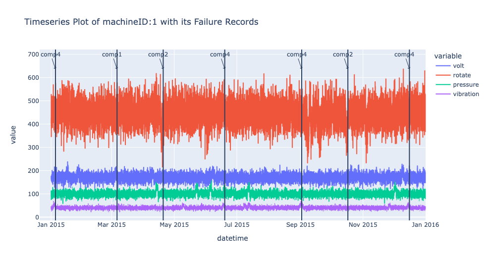
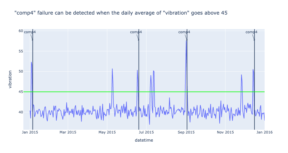
From the following time-series plot where we plotted daily mean value of each sensor, we observe very interesting patterns.
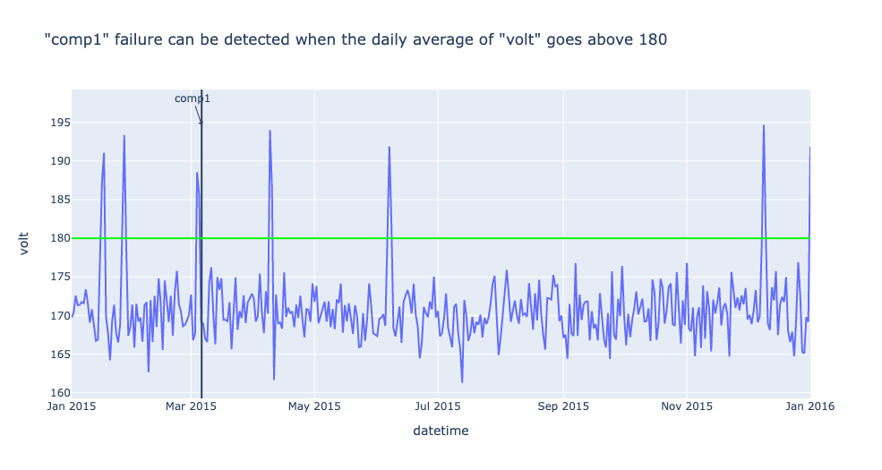
“comp1” failure can be detected when the daily average of “volt” goes above 180
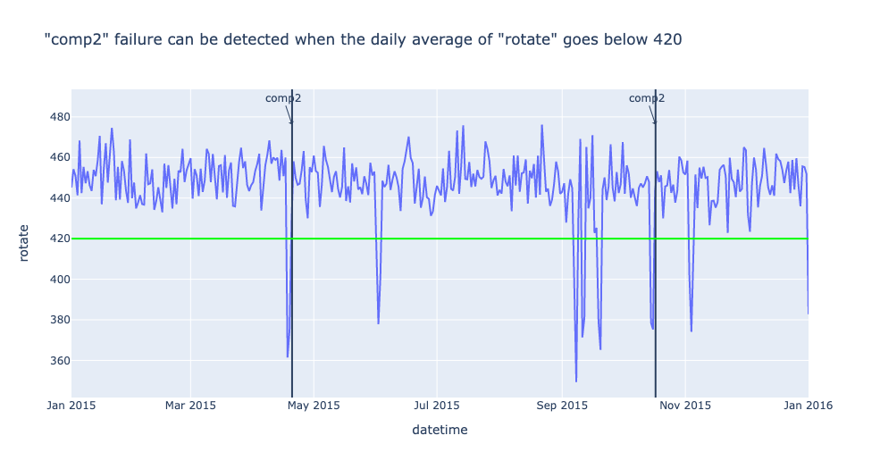
“comp2” failure can be detected when the daily average of “rotate” goes below 420
“comp4” failure can be detected when the daily average of “vibration” goes above 45
df_one_daily = df_one.set_index('datetime').resample('1d').mean()
sensors = 'volt'
fig = px.line(df_one_daily, x=df_one_daily.index, y=sensors,
              title=f'"comp1" failure can be detected when the daily average of "volt" goes above 180')
df_fail_one = df_failures[df_failures.machineID == machine_id]
for row in df_fail_one.iterrows():
    if row[1]['failure'] == 'comp1':
        fig.add_vline(
            row[1]['datetime'],
        )
        fig.add_annotation(x=row[1]['datetime'],
                        y=df_one_daily.max()[sensors],
                        text=row[1]['failure'],
                        showarrow=True,
                        arrowhead=1)
fig.add_hline(180, line_color='#00ff00')
fig.show()
df_one_daily = df_one.set_index('datetime').resample('1d').mean()
sensors = 'rotate'
fig = px.line(df_one_daily, x=df_one_daily.index, y=sensors,
              title=f'"comp2" failure can be detected when the daily average of "rotate" goes below 420')
df_fail_one = df_failures[df_failures.machineID == machine_id]
for row in df_fail_one.iterrows():
    if row[1]['failure'] == 'comp2':
        fig.add_vline(
            row[1]['datetime'],
        )
        fig.add_annotation(x=row[1]['datetime'],
                        y=df_one_daily.max()[sensors],
                        text=row[1]['failure'],
                        showarrow=True,
                        arrowhead=1)
fig.add_hline(420, line_color='#00ff00')
fig.show()
df_one_daily = df_one.set_index('datetime').resample('1d').mean()
sensors = 'vibration'
fig = px.line(df_one_daily, x=df_one_daily.index, y=sensors,
#               hover_data={"date": "|%B %d, %Y"},
              title=f'"comp4" failure can be detected when the daily average of "vibration" goes above 45')
df_fail_one = df_failures[df_failures.machineID == machine_id]
for row in df_fail_one.iterrows():
    fig.add_vline(
        row[1]['datetime'],
    )
    fig.add_annotation(x=row[1]['datetime'],
                       y=df_one_daily.max()[sensors],
                       text=row[1]['failure'],
                       showarrow=True,
                       arrowhead=1)
fig.add_hline(45, line_color='#00ff00')
fig.show()
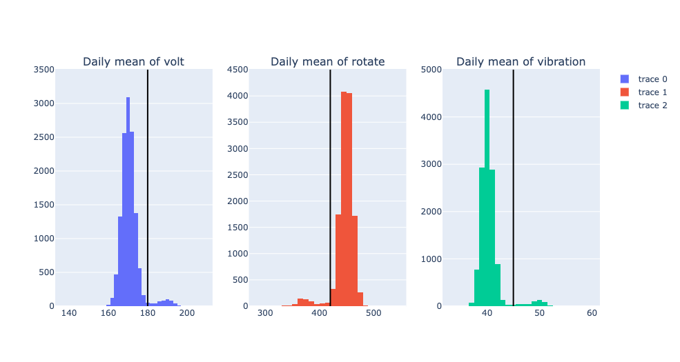
To confirm that these rules are applicable to entire dataset, let’s draw histogram of each sensor using entire model3 machine dataset and see if those thresholds filter out reasonable amount of data.
df_model3['date'] = df_model3['datetime'].apply(lambda x: x.date())
/var/folders/wb/40304xlx477cfjzbk386l2gr0000gn/T/ipykernel_50500/1065329889.py:1: SettingWithCopyWarning:


A value is trying to be set on a copy of a slice from a DataFrame.
Try using .loc[row_indexer,col_indexer] = value instead

See the caveats in the documentation: https://pandas.pydata.org/pandas-docs/stable/user_guide/indexing.html#returning-a-view-versus-a-copy
df_model3_daily = df_model3.groupby(['date', 'machineID']).agg('mean')
df_model3_daily.head()
| volt | rotate | pressure | vibration | age | ||
|---|---|---|---|---|---|---|
| date | machineID | |||||
| 2015-01-01 | 1 | 169.733809 | 445.179865 | 96.797113 | 40.385160 | 18.0 |
| 3 | 170.066825 | 460.956803 | 101.395264 | 37.989643 | 8.0 | |
| 4 | 170.116871 | 440.333823 | 98.378607 | 42.106068 | 7.0 | |
| 5 | 175.674631 | 460.621226 | 97.928488 | 38.591031 | 2.0 | |
| 6 | 166.444305 | 463.516403 | 121.719376 | 38.635407 | 7.0 |
import plotly.graph_objects as go
from plotly.subplots import make_subplots

fig = make_subplots(rows=1, cols=3, subplot_titles=(
                        "Daily mean of volt",
                        "Daily mean of rotate",
                        "Daily mean of vibration"))

trace0 = go.Histogram(x=df_model3_daily['volt'], nbinsx=50)
trace1 = go.Histogram(x=df_model3_daily['rotate'], nbinsx=50)
trace2 = go.Histogram(x=df_model3_daily['vibration'], nbinsx=50)

fig.add_vline(
    row[1]['datetime'],
)

fig.append_trace(trace0, 1, 1)
fig.append_trace(trace1, 1, 2)
fig.append_trace(trace2, 1, 3)

fig.add_shape(type='line',
              x0=180,x1=180,y0=0,y1=3500,
              line=dict(color='Black',),
              row=1,
              col=1)

fig.add_shape(type='line',
              x0=420,x1=420,y0=0,y1=4500,
              line=dict(color='Black',),
              row=1,
              col=2)

fig.add_shape(type='line',
              x0=45,x1=45,y0=0,y1=5000,
              line=dict(color='Black',),
              row=1,
              col=3)
fig.show()
from scipy import stats
percentile1 = stats.percentileofscore(df_model3_daily['volt'], 180)
percentile2 = stats.percentileofscore(df_model3_daily['rotate'], 420)
percentile3 = stats.percentileofscore(df_model3_daily['vibration'], 45)
print(f'percentile of threshold 180 in volt: {percentile1:.3f}')
print(f'percentile of threshold 420 in rotate: {percentile2:.3f}')
print(f'percentile of threshold 45 in vibration: {percentile3:.3f}')
percentile of threshold 180 in volt: 96.081
percentile of threshold 420 in rotate: 4.699
percentile of threshold 45 in vibration: 96.183
From the above histograms, we could confirm that the thresholds we used detect reasonably small portion of dataset as failures.
3.2 Create training / test dataset
We want to create a training and test dataset in this section. We will define one data point as (24,4) array which consists of 4 sensors for 24 hours (daily). We will split training and test data using machineID.
We will use the following three variables in the following sections:
keys: keys will be used to group_by the whole dataset
features: features are the columns that will be used to build models
class_map: class_map will map the faulty component string (ex: ‘comp1’) to integer. ‘non-failure’ will be mapped to integer 0.
keys = ['machineID', 'date']
features = ['volt', 'rotate', 'pressure', 'vibration']
class_map = {'comp1': 1, 'comp2': 2, 'comp4':3}
Remove 2016-01-01 because machine has only one hour data on this date.
import datetime

df_model3 = df_model3[df_model3.date != datetime.datetime(2016, 1, 1).date()]
df_model3.shape
(306600, 9)
Split the entire dataset into Training and Test datasets with split_ratio 3:2
import numpy as np

test_ratio = 0.4
n_split = int(df_model3.machineID.nunique() * test_ratio)
model3_ids = df_model3.machineID.unique()
rng = np.random.default_rng(42)
rng.shuffle(model3_ids)


model3_ids_for_train = model3_ids[n_split:]
model3_ids_for_test = model3_ids[:n_split]
df_model3_train = df_model3[df_model3.machineID.isin(model3_ids_for_train)]
df_model3_test = df_model3[df_model3.machineID.isin(model3_ids_for_test)]
print(df_model3_train.shape, df_model3_test.shape)
(183960, 9) (122640, 9)
Let’s check out how many data points we will have in train and test dataset. Again, each data point will have (24, 4) shape which is (24 hours and 4 features).
temp_gb = df_model3_train.groupby(keys)
list_of_train_daily = [item for item in temp_gb]

temp_gb = df_model3_test.groupby(keys)
list_of_test_daily = [item for item in temp_gb]

print(f'number of data points in train dataset: {len(list_of_train_daily)}')
print(f'number of data points in test dataset: {len(list_of_test_daily)}')
number of data points in train dataset: 7665
number of data points in test dataset: 5110
From the above EDA, we found that failures can be detected one~two days earlier than the recorded date of failure and it is also reasonable to say that there is a one day gap between machine failed date and repair date. So, we will use (recorded repair date - 1 day) as a ground truth date of machine failure.
from datetime import timedelta
df_failures['datetime'] = pd.to_datetime(df_failures['datetime'])
df_failures['date'] = df_failures['datetime'].apply(lambda x: x.date())
df_failures['date_1'] = df_failures['date'] - timedelta(days=1)
Generate ground truth label for train and test datasets. In some failure cases, one machine can have n number of faulty components and, in that case, we generated n data points with n different kinds of labels.
df_failures[(df_failures.machineID==1)]
| datetime | machineID | failure | date | date_1 | |
|---|---|---|---|---|---|
| 0 | 2015-01-05 06:00:00 | 1 | comp4 | 2015-01-05 | 2015-01-04 |
| 1 | 2015-03-06 06:00:00 | 1 | comp1 | 2015-03-06 | 2015-03-05 |
| 2 | 2015-04-20 06:00:00 | 1 | comp2 | 2015-04-20 | 2015-04-19 |
| 3 | 2015-06-19 06:00:00 | 1 | comp4 | 2015-06-19 | 2015-06-18 |
| 4 | 2015-09-02 06:00:00 | 1 | comp4 | 2015-09-02 | 2015-09-01 |
| 5 | 2015-10-17 06:00:00 | 1 | comp2 | 2015-10-17 | 2015-10-16 |
| 6 | 2015-12-16 06:00:00 | 1 | comp4 | 2015-12-16 | 2015-12-15 |
x_train_list = []
y_train_list = []
for idx, df_daily_one in list_of_train_daily:
    mid = idx[0]
    date = idx[1]

    if df_daily_one.shape[0] != 24:
        continue

    df_filtered_f = df_failures[(df_failures.date_1==date)&(df_failures.machineID==mid)]
    if df_filtered_f.shape[0] >= 1:
        for i in range(df_filtered_f.shape[0]):
            x_train_list.append(df_daily_one[keys+features])
            y_train_list.append(class_map[df_filtered_f['failure'].iloc[i]])
    else:
        x_train_list.append(df_daily_one[keys+features])
        y_train_list.append(0)

# x_whole = np.stack(x_list, 0)
# y_whole = np.array(y_true_list)
print('len(x_train_list):', len(x_train_list), x_train_list[0].shape)
print('len(y_train_list):', len(y_train_list))
len(x_train_list): 7667 (24, 6)
len(y_train_list): 7667
x_test_list = []
y_test_list = []
for idx, df_daily_one in list_of_test_daily:
    mid = idx[0]
    date = idx[1]

    if df_daily_one.shape[0] != 24:
        continue

    df_filtered_f = df_failures[(df_failures.date_1==date)&(df_failures.machineID==mid)]
    if df_filtered_f.shape[0] >= 1:
        for i in range(df_filtered_f.shape[0]):
            x_test_list.append(df_daily_one[keys+features])
            y_test_list.append(class_map[df_filtered_f['failure'].iloc[i]])
    else:
        x_test_list.append(df_daily_one[keys+features])
        y_test_list.append(0)

# x_whole = np.stack(x_list, 0)
# y_whole = np.array(y_true_list)
print('len(x_test_list):', len(x_test_list), x_test_list[0].shape)
print('len(y_test_list):', len(y_test_list))
len(x_test_list): 5117 (24, 6)
len(y_test_list): 5117
Check out the distribution of ground truth labels in test dataset. In ideal case, dataset should have a balanced classes.
unique, counts = np.unique(y_train_list, return_counts=True)
print(np.asarray((unique, counts)).T)
[[   0 7531]
 [   1   45]
 [   2   55]
 [   3   36]]
unique, counts = np.unique(y_test_list, return_counts=True)
print(np.asarray((unique, counts)).T)
[[   0 5032]
 [   1   23]
 [   2   34]
 [   3   28]]
4. Build a rule-based model
4.1 Build a rule-based model that can predict the faulty component of a machine
In the previous section, we have found following rules that can detect the faulty component of a machine.
“comp1” failure can be detected when the daily average of “volt” goes above 180
“comp2” failure can be detected when the daily average of “rotate” goes below 420
“comp4” failure can be detected when the daily average of “vibration” goes above 45
Now, using these three rules, let’s build a simple rule-based model that can classify three different kinds of component failures of model3 machines.
from dataclasses import dataclass

@dataclass
class RuleModel:
    daily_thresholds = {
        'volt': 180, # >
        'rotate': 420, # <
        'vibration': 45, # >
    }

    def predict(self, input_data):
        df = input_data['X']
        df_resampled = df.mean(axis=0)

        results = {'predictions': 0}
        if df_resampled['volt'] > self.daily_thresholds['volt']:
            results['predictions'] = 1
        if df_resampled['rotate'] < self.daily_thresholds['rotate']:
            results['predictions'] = 2
        if df_resampled['vibration'] > self.daily_thresholds['vibration']:
            results['predictions'] = 3
        return results
4.2 Evaluate the performance of the rule-based model
Using the test dataset we generated in #3.2, let’s evaluate the performance of rule-based Fault Predictor
rule_model = RuleModel()
y_rule_model_list = []
for x_test in x_test_list:
    rule_model_pred = rule_model.predict({
        'X': x_test[features]
    })['predictions']
    y_rule_model_list.append(rule_model_pred)
from sklearn import metrics
cm_rule_based = metrics.confusion_matrix(y_test_list, y_rule_model_list)
cm_rule_based
array([[4519,  149,  194,  170],
       [   0,   20,    1,    2],
       [   0,    0,   29,    5],
       [   0,    0,    0,   28]])
f1_micro_rule_model = metrics.f1_score(y_test_list, y_rule_model_list, average='micro')
f1_macro_rule_model = metrics.f1_score(y_test_list, y_rule_model_list, average='macro')

print(f'f1_micro_rule_model: {f1_micro_rule_model:.3f}', f'f1_macro_rule_model: {f1_macro_rule_model:.3f}')
f1_micro_rule_model: 0.898 f1_macro_rule_model: 0.405
def get_precision_n_recall_per_class(cm, n_class):
    list_f1 = []
    for cls in range(n_class):
        precision = cm[cls, cls]/sum(cm[:, cls])
        recall = cm[cls, cls]/sum(cm[cls, :])
        f1 = 2 * (precision*recall) / (precision+recall)
        list_f1.append(f1)
        print(f"class: {cls}, precision: {precision:.3f}, recall: {recall:.3f}, f1_score: {f1:.3f}")
    print(f"Average F1 Score: {sum(list_f1)/len(list_f1):.3f}")
get_precision_n_recall_per_class(cm_rule_based, n_class=4)
class: 0, precision: 1.000, recall: 0.898, f1_score: 0.946
class: 1, precision: 0.118, recall: 0.870, f1_score: 0.208
class: 2, precision: 0.129, recall: 0.853, f1_score: 0.225
class: 3, precision: 0.137, recall: 1.000, f1_score: 0.240
Average F1 Score: 0.405
From the above evaluate results, we can find that this simple rule-based model can detect the faulty component of machine with pretty high recalls. We can also find that the precision of this model is very low and we can say this model detects many of normal machine as failed machines (gives many false alarm).
5. Build an Oracle using H1st.TimeSeriesOracle
5.1 Build an Oracle from a rule-based Fault Predictor
from h1st.model.oracle.ts_oracle_modeler import TimeseriesOracleModeler
from h1st.model.oracle.student import RandomForestModeler, AdaBoostModeler
from h1st.model.rule_based_modeler import RuleBasedModeler
from h1st.model.rule_based_model import RuleBasedClassificationModel

oracle_modeler = TimeseriesOracleModeler(teacher=RuleModel(),
    student_modelers = [RandomForestModeler(), AdaBoostModeler()],
    ensembler_modeler = RuleBasedModeler(model_class=RuleBasedClassificationModel)
    )

oracle = oracle_modeler.build_model(
    data={'unlabeled_data': df_model3_train[keys+features]},
    id_col='machineID',
    ts_col='date'
)
5.2 Evaluate the performance of Oracle and compare it with that of rule-based model
y_oracle_list = []
for x_test in x_test_list:
    oracle_pred = oracle.predict({
        'X': x_test[keys+features]
    })['predictions'][0]
    y_oracle_list.append(oracle_pred)
from sklearn import metrics
cm_oracle = metrics.confusion_matrix(y_test_list, y_oracle_list)
cm_oracle
array([[4641,   79,  154,  158],
       [   6,   15,    0,    2],
       [   2,    1,   26,    5],
       [   0,    0,    0,   28]])
get_precision_n_recall_per_class(cm_oracle, n_class=4)
class: 0, precision: 0.998, recall: 0.922, f1_score: 0.959
class: 1, precision: 0.158, recall: 0.652, f1_score: 0.254
class: 2, precision: 0.144, recall: 0.765, f1_score: 0.243
class: 3, precision: 0.145, recall: 1.000, f1_score: 0.253
Average F1 Score: 0.427
f1_micro_oracle = metrics.f1_score(y_test_list, y_oracle_list, average='micro')
f1_macro_oracle = metrics.f1_score(y_test_list, y_oracle_list, average='macro')

print(f'f1_micro_oracle: {f1_micro_oracle:.3f}', f'f1_macro_oracle: {f1_macro_oracle:.3f}')
f1_micro_oracle: 0.920 f1_macro_oracle: 0.427
print(f'f1_micro_rule_model: {f1_micro_rule_model:.3f}', f'f1_macro_rule_model: {f1_macro_rule_model:.3f}')
f1_micro_rule_model: 0.898 f1_macro_rule_model: 0.405
From the above test results, we can see that Oracle made improvement in both f1_micro and f1_macro around 2.3% and 3.4% compared to the f1 score of rule-based model.
Test out if a persisted Oracle can be loaded and give the same predictions as the original Oracle object.
import os
import tempfile

from h1st.model.oracle import TimeSeriesOracle
from h1st.model.oracle.student import RandomForestModel, AdaBoostModel

with tempfile.TemporaryDirectory() as path:
    os.environ['H1ST_MODEL_REPO_PATH'] = path
    version = oracle.persist()

oracle_2 = TimeSeriesOracle(teacher=RuleModel(),
                            students= [RandomForestModel(), AdaBoostModel()],
                            ensembler=RuleBasedClassificationModel())
oracle_2.load_params(version)
y_oracle_loaded_list = []
for x_test in x_test_list:
    oracle_pred = oracle_2.predict({
        'X': x_test[keys+features]
    })['predictions'][0]
    y_oracle_loaded_list.append(oracle_pred)
f1_micro_oracle_loaded = metrics.f1_score(y_test_list, y_oracle_loaded_list, average='micro')
f1_macro_oracle_loaded = metrics.f1_score(y_test_list, y_oracle_loaded_list, average='macro')

print(f'f1_micro_oracle_loaded: {f1_micro_oracle_loaded:.3f}', f'f1_macro_oracle_loaded: {f1_macro_oracle_loaded:.3f}')
f1_micro_oracle_loaded: 0.920 f1_macro_oracle_loaded: 0.427
From the above evaluation results, we could confirm that the loaded Oracle provides the same results. Using this .persist() and .load() mechanism, you can easily reuse the built Oracle in real-world applications.
6. Summary
In this tutorial, we have achieved the following: 1. We could understand what is H1st Oracle and how to build it from Rule-based Model (encoding expert knowledge) and unlabeled data. 2. We could evaluate the performance of H1st Oracle and rule-based Model and found that Oracle outperforms the rule-based model even though we haven’t used any labeled data to build Oracle. This is because Oracle includes discriminative models that can generalize the encoded rules of rule-based model and, furthermore, combine their intelligence through ensemble.
We hope you enjoyed this tutorial. You can find the notebook version of this tutorial here. To find more information about H1st, please visit our h1st website or check out our h1st github repository. See you again-!